3D Scanner
a point cloud generator
Overview
For my introductory electrical engineering course final project, I chose to make a 3D scanner. The scanner mapped contours of objects from the measurements of an infrared time of flight distance sensor. Data from multiple contours was then parsed and compiled to generate point clouds in MATLAB. The process of measuring contours was coordinated by an Arduino UNO.
Design
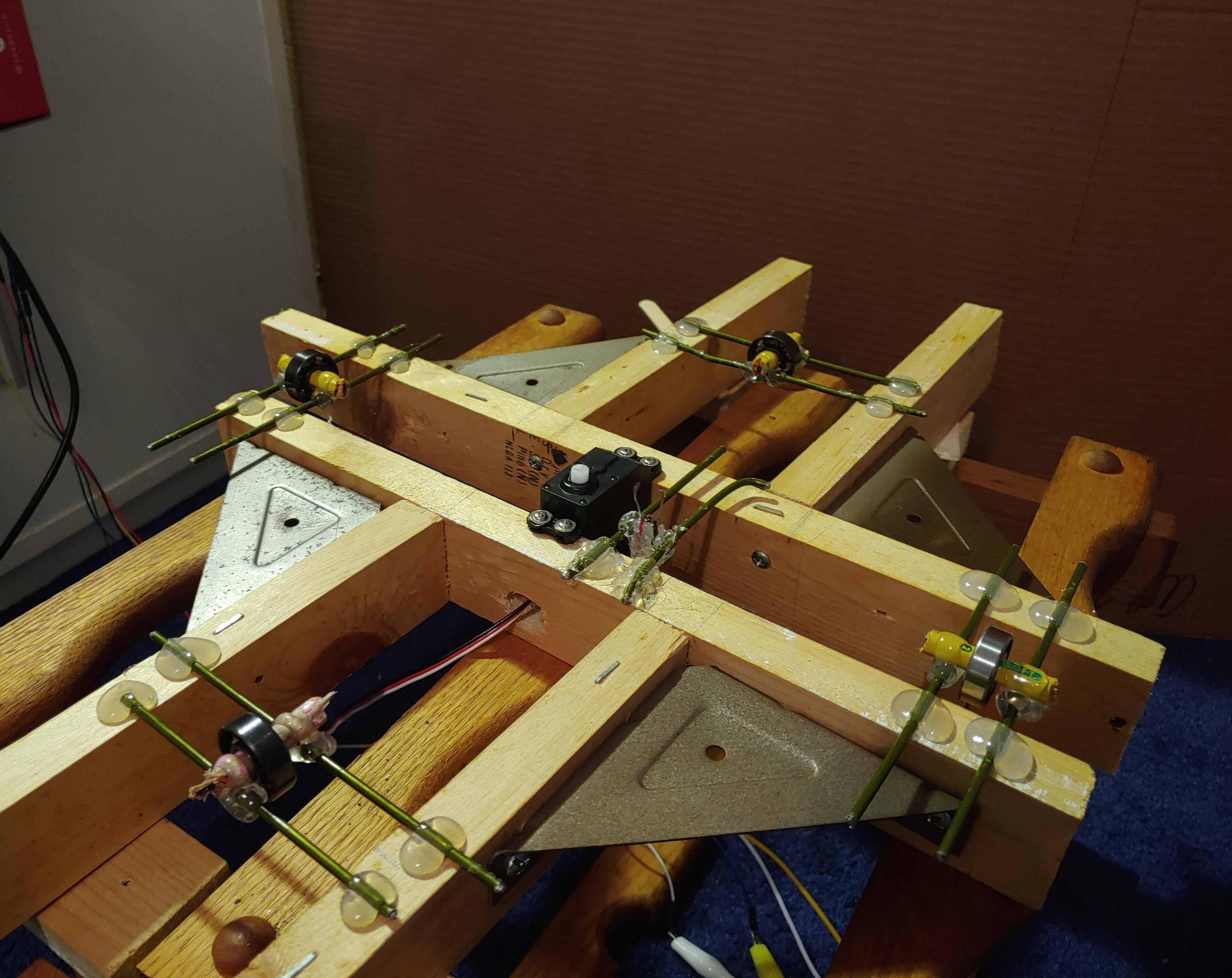
The design centered on a VL53L1X infrared time of flight (ToF) sensor. The sensor was mounted to a sliding track to fix its X-Y position while taking different contours. Objects to be scanned were placed on a platform driven by a continuous servo, which guided the object through 5 revolutions as distance measurements were taken. Each contour was written to a an SD card as a text file with the Z-position included in its name.
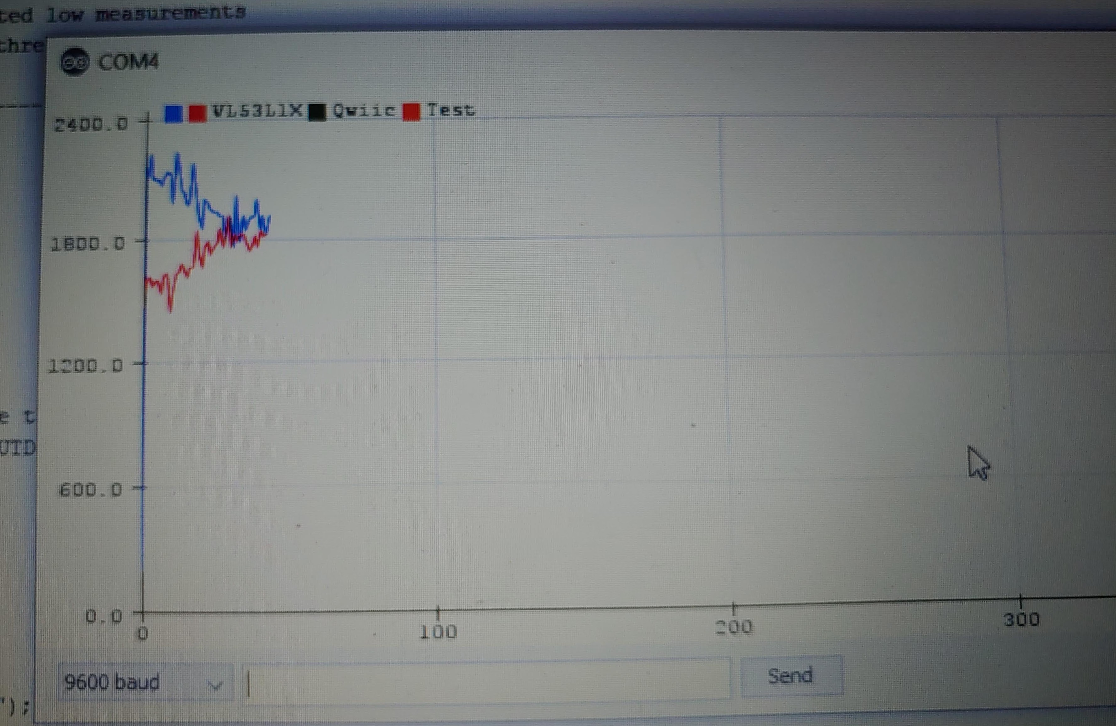
In order to generate contours from the distance measurements, the position of the revolution axis relative to the ToF sensor must be known. This information was gathered through supporting alignment and range finding programs. The alignment program, which was run prior to taking contours, measured the time a thin rod spent on the left and right sides of the ToF sensor when mounted to the servo platform. I adjusted the optical center of the VL53L1X’s photodiode array to equalize these times, such that it pointed to the revolution axis. The rangefinder program averaged 98 distance readings to a flat surface perpendicular to the ToF sensor’s line of sight and intersecting the revolution axis to find the distance to the axis.

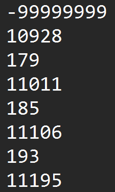
The angular position of distance readings must also be known to generate contours. A continuous servo controlled the target objects’ angular velocity and allowed multiple revolutions while remaining within budget constraints. It did not, however, directly control the angular position as a standard servo, or stepper motor would have. Rotations were instead tracked by attaching a conductive pin to the servo platform’s underside which closed a circuit at the end of each revolution. Revolutions were marked in distance measurement files by a nonphysical “-99999999” reading.
Contour generation was completed by a MATLAB script which read the distance measurement files, parsing out revolution markers. The script interpolated the angular position of each distance reading within a revolution assuming constant angular velocity. After parsing all contours of an object, another script compiled them into a list of coordinates with Z-positions retrieved from the file names. The point cloud was then viewable as a 3D scatter plot.